Tensile Testing: Stress-Strain Curves, Key Parameters, and Standards
Tensile testing is the single most widely performed mechanical test in metallic materials characterisation. By pulling a standardised specimen to fracture under controlled conditions, it simultaneously quantifies elastic stiffness, yield behaviour, strain-hardening capacity, ultimate strength, and ductility — providing the primary dataset that underpins structural design codes, weld procedure qualification, material acceptance inspection, and failure analysis across virtually every engineering industry.
Key Takeaways
- Engineering stress uses original area (A0); true stress uses instantaneous area — the two diverge significantly beyond the UTS.
- Young’s modulus (E) is a structure-insensitive property determined solely by atomic bonding; for steel it is approximately 200–210 GPa regardless of heat treatment.
- The 0.2% proof stress (Rp0.2) is the internationally accepted yield criterion for alloys lacking a defined yield point.
- Necking initiates when the work-hardening rate equals the current true stress (Considère criterion: dσ/dε = σ).
- ASTM E8/E8M and ISO 6892-1 govern room-temperature tensile testing; ISO 6892-2 covers elevated-temperature testing.
- Percentage elongation depends on gauge length; comparison is only valid between proportional specimens (L0 = 5.65√A0 or 11.3√A0).
Fundamental Principles of the Tensile Test
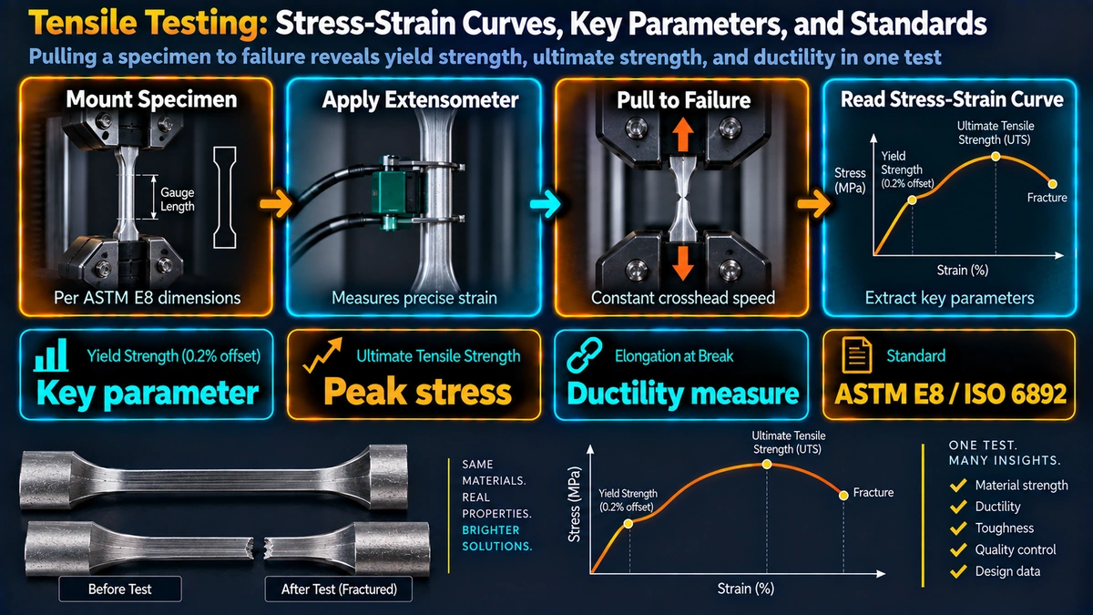
In a standard tensile test, a machined specimen of defined geometry is gripped at both ends and subjected to a progressively increasing uniaxial tensile force at a controlled crosshead displacement rate or strain rate. Load and extension are continuously recorded, typically by a load cell and a clip-on extensometer or a non-contacting video extensometer. The resulting load-extension data are normalised to stress and strain using the original specimen dimensions, producing the engineering stress-strain curve.
Engineering Stress and Engineering Strain
Engineering (nominal) stress and strain are defined with reference to the original, undeformed gauge section:
σe = F / A₀

εe = (L - L₀) / L₀ = ΔL / L₀
where F is the applied force (N), A0 is the original cross-sectional area (mm²), L is the current gauge length (mm), and L0 is the original gauge length (mm). Engineering stress is reported in MPa (N/mm²) and engineering strain as a dimensionless ratio (or percentage for elongation calculations).
True Stress and True Strain
The engineering convention ignores the continuous reduction in cross-section as the material deforms. True (Cauchy) stress and true (logarithmic or Hencky) strain correct for this:
σT = F / Ai   (Ai = instantaneous cross-sectional area)

εT = ln(L / L₀) = ln(1 + εe)

Before necking, using volume conservation (AiL = A₀L₀):
σT = σe(1 + εe)
εT = ln(1 + εe)
These conversions are valid only up to the onset of necking. Beyond necking, the deformation is no longer uniform along the gauge length, and true stress must be calculated from instantaneous area measurements combined with the Bridgman correction for triaxial stress state within the neck.
The Stress-Strain Curve — Region by Region
1. Elastic Region and Young’s Modulus
From zero load to the elastic limit, stress and strain are linearly proportional — Hooke’s Law holds. The gradient of this linear region is Young’s modulus (modulus of elasticity), E:
E = σ / ε (in the linear elastic region, units: GPa)Young’s modulus is a structure-insensitive property controlled by interatomic bonding force rather than microstructure or heat treatment. For iron and carbon steels, E ≈ 200–210 GPa at room temperature. Alloying has only minor effects; cold work and heat treatment have essentially no effect. In contrast, grain size and dislocation density do not alter E.
The elastic region is recoverable: if load is removed anywhere before the elastic limit, the specimen returns to its original dimensions with no permanent set.
2. Yield Behaviour
Discontinuous Yielding in Mild Steel
Mild steels (low-carbon ferritic steels) exhibit a sharply defined upper yield point (σUY) followed by a drop to the lower yield point (σLY). This discontinuous yielding is caused by the locking of dislocations by Cottrell atmospheres — segregation of interstitial carbon and nitrogen atoms to dislocation cores. The upper yield stress is the stress to unpin dislocations; once unpinned, they propagate at a lower applied stress.
Following the yield drop, localised deformation bands (Lüders bands, also called Hartmann lines or stretcher strains) nucleate near stress concentrations and propagate along the specimen at roughly constant stress, producing the flat yield plateau on the engineering curve. Lüders bands are visible as surface markings on polished specimens and are responsible for the “fluting” surface defect in press-formed mild steel panels.
Continuous Yielding and the 0.2% Proof Stress
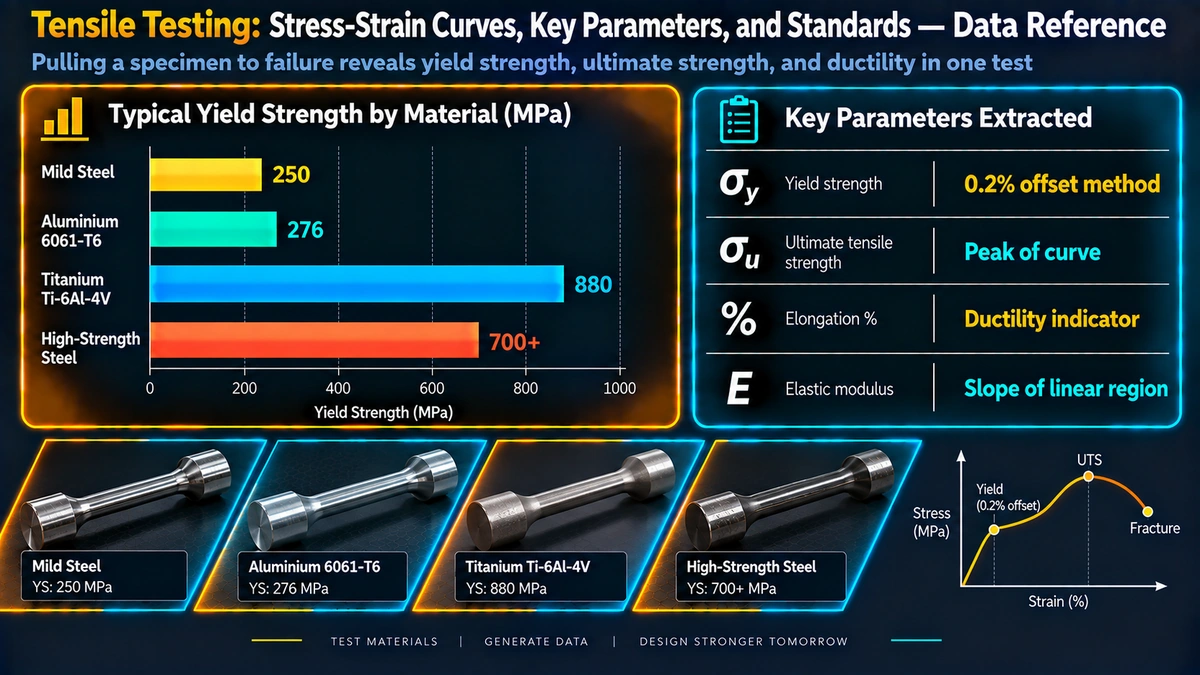
Most engineering alloys — including high-strength steels, aluminium alloys, austenitic stainless steels, copper alloys, and titanium alloys — show a gradual, continuous transition from elastic to plastic behaviour with no distinct yield point. For these materials, yield strength is quantified as the 0.2% proof stress (Rp0.2), defined by the intersection of the stress-strain curve with a line drawn parallel to the elastic slope but offset by 0.002 (0.2%) plastic strain:
Method: Draw a line from ε = 0.002 with slope E.
The intersection with the σ-ε curve = Rp0.2 (0.2% proof stress)
Other proof stress levels are also used: Rp0.1 (0.1% offset) is common in aerospace aluminium alloys; Rp1.0 (1.0% offset) or Rt0.5 (total strain at 0.5%) appear in pressure vessel codes. The relevant design standard specifies which quantity applies.
3. Strain Hardening (Work Hardening) Region
Beyond yield, continued plastic deformation requires increasing stress — the material strain hardens. Strain hardening results from dislocation multiplication and the increasing difficulty of dislocation motion as dislocation density rises and short-range obstacles (forest dislocations, solute atoms, precipitates, grain boundaries as in the Hall-Petch relationship) increase.
The power-law (Hollomon) equation describes the true stress-strain relationship in the plastic region for many metals:
σT = K εTn

K = strength coefficient (MPa)
n = strain-hardening exponent (dimensionless, 0 < n < 1)

Typical n values:
  Low-carbon steel:        n ≈ 0.20 – 0.26
  Austenitic stainless:    n ≈ 0.40 – 0.55
  Aluminium alloy (5xxx):  n ≈ 0.15 – 0.25
  Copper (annealed):       n ≈ 0.35 – 0.45
A high n value indicates strong strain hardening and good formability in deep-drawing operations (see hardness testing for complementary property data). The n value is measured from log-log plots of true stress vs. true strain in the uniform plastic region.
4. Ultimate Tensile Strength (UTS) and Onset of Necking
The engineering stress peaks at the UTS (Rm in ISO notation, Fu/A0). At this point, the material’s ability to strain-harden can no longer compensate for the geometrical softening from cross-section reduction. The Considère criterion defines this instability:
Neck initiates when:  dσT/dεT = σT

In terms of engineering quantities, UTS engineering strain εu = n
(for a Hollomon material: the uniform elongation equals the strain-hardening exponent)
Beyond the UTS, deformation concentrates in a local neck. The cross-section in the neck falls rapidly, so engineering stress (F/A0) drops even as true stress (F/Ai) continues to rise. Neck geometry evolves toward a roughly elliptical cross-section in round specimens; in flat specimens, a diffuse neck (in width) followed by a through-thickness shear localisation is typical.
5. Fracture
Ductile fracture in metallic materials initiates by nucleation of voids at second-phase particles, inclusions, or grain boundary triple points within the neck. Voids grow and coalesce through localised plastic deformation, forming an internal crack that propagates by a repeated void-coalescence mechanism. The macroscopic result in round specimens is the characteristic cup-and-cone fracture morphology: a flat, fibrous central region (Mode I void coalescence) surrounded by an inclined shear lip (45° shear fracture). Scanning electron microscopy of the fracture surface reveals dimpled rupture microvoids whose diameter and depth reflect the void nucleation site spacing.
Brittle fracture (cleavage or intergranular) in tensile tests is associated with reduced temperature, hydrogen embrittlement, temper embrittlement, or material defects. In cleavage fracture, the fracture surface shows facets aligned with crystallographic cleavage planes {100} in BCC iron, producing a bright, granular, faceted appearance. For further discussion of embrittlement mechanisms, see the article on hydrogen-induced cracking.
Key Mechanical Parameters Extracted from the Tensile Test
| Parameter | Symbol (ISO/ASTM) | Definition | Typical steel range |
|---|---|---|---|
| Young’s modulus | E / E | Slope of initial linear elastic region | 195–215 GPa |
| 0.2% proof stress | Rp0.2 / YS | Stress at 0.2% plastic offset | 200–1800 MPa |
| Upper yield strength | ReH / UYS | Peak stress before yield drop (mild steel) | 250–350 MPa |
| Lower yield strength | ReL / LYS | Stress at Lüders band propagation | 230–320 MPa |
| Ultimate tensile strength | Rm / UTS | Maximum engineering stress; load at necking onset | 350–2200 MPa |
| % Elongation after fracture | A / %El | (Lf-L0)/L0 × 100 | 5–50% |
| % Reduction of area | Z / RA | (A0-Af)/A0 × 100 | 30–75% |
| Strain-hardening exponent | n | Hollomon exponent fitted to true σ-ε curve | 0.10–0.55 |
Percentage Elongation and Gauge Length Dependence
Percentage elongation (A) combines uniform elongation (distributed through the whole gauge) and localised elongation (concentrated in the neck). Because the localised component is a fixed physical length, shorter gauge lengths L0 yield higher A values for the same material. This is why elongation results must always be reported together with gauge length, and comparisons are only valid between specimens with the same ratio L0/√A0 (proportionality coefficient k):
ISO standard proportional gauge lengths:
  Round specimen: L₀ = 5.65√A₀  (equivalent to 5d₀ for circular section)
  Flat specimen:  L₀ = 5.65√(b₀ × t₀)

ASTM standard gauge lengths (fixed):
  Sub-size:       L₀ = 1.000 in (25.4 mm)
  Standard:       L₀ = 2.000 in (50.8 mm)
Reduction of Area
Reduction of area Z (or RA) is independent of gauge length, making it the preferred ductility measure for detecting embrittlement:
Z (%) = (A₀ - Af) / A₀ × 100

A₀ = original cross-sectional area
Af = minimum cross-sectional area at fracture location
RA is especially sensitive to hydrogen embrittlement (see hydrogen-induced cracking in steel), temper embrittlement, and low test temperature. Specification limits for RA are common in high-strength steel qualifications for oil and gas sour service per NACE MR0175/ISO 15156.
Tensile Testing Standards: ASTM E8 and ISO 6892
ASTM E8/E8M
ASTM E8 (customary units) and E8M (SI units) govern tensile testing of metallic materials at room temperature in the USA. The standard prescribes specimen geometries (round and flat, standard and sub-size), gripping methods, extensometer classification (ISO 9513 Class B1 or better for yield measurement), stress rate in the elastic range, and strain rate in the plastic range. The standard permits a stress rate of 1.15–11.5 MPa/s in the elastic range and specifies that strain rate in the plastic range shall not exceed 0.5 mm/(mm⋅min) for yield properties.
ISO 6892-1
ISO 6892-1 (room temperature) is the European and international equivalent. Its critical advance over earlier editions was the introduction of strain-rate-controlled testing methods to reduce the influence of the testing machine’s stiffness on reported yield strength:
| Method | Control mode | Notes |
|---|---|---|
| Method A (A1/A2) | Closed-loop strain rate control via extensometer feedback | Preferred; minimises machine compliance effects; A1 lower rate, A2 higher rate |
| Method B | Crosshead separation rate (estimated strain rate) | Acceptable where Method A not available; relies on machine stiffness correction |
ISO 6892-2 covers elevated-temperature tensile testing. The companion standard ISO 148-1 governs Charpy impact testing, and ISO 6507 covers Vickers hardness.
Strain Rate Sensitivity
Yield strength and UTS increase with increasing strain rate for most metals (positive strain rate sensitivity). The Cowper-Symonds relation describes this for high-rate events:
σ_y(ḝ) = σ_y0 [1 + (ḝ/C)^(1/p)]

ḝ = strain rate (s⁻¹)
C, p = material-dependent Cowper-Symonds constants
Example for mild steel: C ≈ 40.4 s⁻¹, p ≈ 5
For standard quasi-static tensile testing the strain rate effect is small, but interlaboratory round robins demonstrate that uncontrolled crosshead speed leads to systematically different yield strength results — hence the ISO 6892-1 Method A requirement.
Specimen Geometry and Preparation
Round Specimens
Round (cylindrical gauge) specimens are preferred for isotropic materials. Standard ASTM E8M round specimen dimensions are: gauge diameter d0 = 12.5 mm, gauge length L0 = 50 mm. ISO proportional round specimens use d0 = 10 mm or 8 mm with L0 = 5d0. The transition radius between gauge section and shoulders must be at least 8–12 mm to avoid stress concentration at the fillet. Surface finish Ra ≤ 1.6 μm is typically required in the gauge length.
Flat (Sheet) Specimens
Flat specimens are used for thin sheet and strip material, and for testing in specified orientations relative to rolling direction (0°, 45°, 90° for anisotropy characterisation). Flat specimens are also used for weld procedure qualification in transverse tensile tests, where the full weld cross-section must be included in the gauge width. Width reduction at shoulders must provide smooth streamlined transitions to avoid corner cracking.
Machining and Surface Finish
All cutting and grinding must be done with sufficient coolant to prevent localised heating and microstructural alteration. Final machining should be in the direction of the gauge length axis to avoid circumferential tool marks that act as stress raisers. Specimens with visible machining damage, burrs, or surface cracks must be rejected before testing.
Special Phenomena on the Stress-Strain Curve
Portevin-Le Chatelier (PLC) Effect — Serrated Flow
Certain alloys, particularly Al-Mg alloys (5xxx series), Al-Cu alloys, and austenitic stainless steels at specific temperature-strain rate combinations, exhibit serrated (jerky) flow — a series of stress drops superimposed on the general work-hardening curve. This is the Portevin-Le Chatelier (PLC) effect, arising from dynamic strain ageing: mobile dislocations are temporarily trapped by diffusing solute atoms, then break free, then are re-pinned. The critical condition is that the dislocation waiting time at an obstacle matches the diffusion time for solute atoms to segregate to the arrest site. PLC effect produces visible surface markings (PLC bands) and may impair formability, surface quality, and fatigue resistance.
Yield Point Return (Strain Ageing)
If a mild steel specimen is deformed into the plastic region, unloaded, and re-tested after storage at room temperature (or brief heating), the yield point phenomenon can re-appear — often at a higher level than the original upper yield point. This yield point return is caused by re-segregation of carbon/nitrogen atoms to dislocations during ageing. Static strain ageing is exploited in the production of high-strength bainitic steels and can cause problems in the press-forming of pre-strained automotive sheet.
Bauschinger Effect
If a material is plastically deformed in tension and then compressed, the compressive yield stress is lower than it would be for a virgin (undeformed) specimen. This is the Bauschinger effect, attributed to residual internal back-stresses built up by heterogeneous dislocation pile-ups at obstacles during forward loading. The Bauschinger effect is important for cyclic loading, springback prediction in forming, and residual stress analysis after autofrettage or straightening operations.
Anisotropy: Lankford Parameter (r-value)
For sheet metals used in deep drawing, the anisotropy of plastic flow is quantified by the Lankford parameter (r-value or plastic strain ratio):
r = ε_w / ε_t

ε_w = true plastic strain in the width direction
ε_t = true plastic strain in the thickness direction

r = ln(w/w₀) / ln(t/t₀)   (measured at ~15-20% elongation)

r-bar (normal anisotropy) = (r₀ + 2r₄₅ + r₉₀) / 4
Δr (planar anisotropy) = (r₀ - 2r₄₅ + r₉₀) / 2
High r-bar (r > 1) indicates resistance to thinning and good deep-drawing performance. Low Δr indicates uniform in-plane properties and minimises earing in drawn cups. Measurements at 0°, 45°, and 90° to the rolling direction are required. The steel industry invests heavily in texture control (alloying and thermomechanical processing) to maximise r-bar in deep-drawing grades.
Tensile Testing in Weld Procedure Qualification
Weld procedure qualification under ASME Section IX (QW-150), AWS D1.1 (clause 4.8), and ISO 15614-1 requires transverse tensile testing of welded test assemblies. The test specimen spans the full weld cross-section (weld metal + both HAZ regions + parent material); the weld crown and root are normally machined flush. Acceptance requires:
ASME Section IX QW-153:
  Tensile strength ≥ minimum specified tensile strength of base metal
  (Failure in weld metal is acceptable if strength requirement is met)

ISO 15614-1 Clause 7.4.3:
  R_m ≥ minimum R_m of base metal per material standard
  Location of fracture must be recorded
Longitudinal weld tensile tests (AWS B4.0, ISO 4136) evaluate weld metal properties independently and are used for filler metal qualification and deposit property verification. For further detail on heat-affected zone microstructure and properties, see the HAZ microstructure guide.
Elevated-Temperature Tensile Testing
ISO 6892-2 and ASTM E21 govern tensile testing at elevated temperatures (typically up to 1200°C for refractory metals). Critical additional requirements include furnace temperature uniformity (±2°C across gauge per ISO 6892-2), thermal soaking time before loading, use of high-temperature extensometers (contact rod type or optical), and inert atmosphere or vacuum to prevent oxidation for reactive metals. Elevated-temperature tensile data are used to define creep rupture design allowables (ASME Section II Part D), hot-working parameter maps, and creep and stress rupture life prediction.
Tensile Strength Estimation from Hardness
When tensile testing is not feasible (e.g., small components, in-service assessment), hardness-to-tensile-strength conversion provides a practical estimate. For carbon and low-alloy steels:
UTS (MPa) ≈ 3.3 × HV  (ferritic/pearlitic steels, HV 100–350)
UTS (MPa) ≈ 3.45 × HBW  (carbon steels, HBW 100–350)

These approximations are less reliable for:
  - Quenched and tempered steels (QT)
  - Austenitic stainless steels
  - Aluminium alloys (use alloy-specific curves)
  - Cold-worked materials
The hardness testing guide covers Vickers, Brinell, Rockwell, and portable Leeb/UCI methods. For fast material identification and tensile strength estimation in the field, the MetallurgyZone calculators hub provides hardness-to-UTS conversion tools.
Industrial Applications
Tensile testing underpins materials certification and process control across all engineering sectors:
- Structural steel production: Every heat of structural steel (e.g., EN 10025, ASTM A36, API 2W) requires tensile and Charpy certification before despatch — see also the Charpy impact testing guide.
- Pressure vessel fabrication: Base material certification and weld procedure qualification per ASME VIII, EN 13445, or PD 5500.
- Oil and gas pipelines: API 5L requires full-body tensile (longitudinal and transverse), weld seam transverse tensile, and guided bend tests for each pipe.
- Aerospace structures: MIL-HDBK-5 (now MMPDS) design allowables are derived from large statistical tensile test databases; AS9100 traceability requirements apply to every test coupon.
- Automotive sheet steel: AHSS (dual-phase, TRIP, TWIP, martensitic) grades are characterised by their tensile curve shape: high n-value, high elongation product (UTS × total elongation > 20,000 MPa·%).
- Post-weld heat treatment (PWHT) qualification: PWHT simulation coupons are tensile-tested to verify that the required strength and toughness are maintained after the thermal cycle — see the article on annealing and normalising.
Frequently Asked Questions
What is the difference between engineering stress and true stress?
How is the 0.2% proof stress (offset yield strength) determined?
Why do mild steels show an upper and lower yield point?
What governs the onset of necking in a tensile test?
What is the Portevin-Le Chatelier effect?
What are the key differences between ASTM E8/E8M and ISO 6892-1?
How does specimen geometry affect tensile test results?
What is reduction of area and what does it indicate?
How is tensile testing used for weld procedure qualification?
Can tensile strength be reliably estimated from hardness measurements?
Recommended Reference Books
Further Reading
