Fatigue Life Calculator (S-N Curve Based)
Predicting fatigue life starts with an S-N curve — the empirical relationship between applied stress and cycles to failure. This calculator estimates fatigue life two ways: by fitting a power-law curve through two known S-N data points, or by applying Basquin’s equation directly from a material’s fatigue strength coefficient and exponent. The article below covers the underlying theory, its limitations, and how it connects to cumulative damage analysis.
Key Takeaways
- S-N curves plot stress against cycles to failure on a log-log basis because fatigue life spans orders of magnitude for a modest stress range.
- The two-point method fits S = A x N^b through any two known data points on a material’s S-N curve.
- Basquin’s equation, Sa = sigma_f’ x (2Nf)^b, uses standardized fatigue strength properties instead of raw test points.
- Many steels exhibit a fatigue (endurance) limit — a stress plateau below which life is effectively infinite — that a single power-law fit does not automatically capture.
- S-N based life predictions carry substantial inherent scatter and are best used comparatively, not as a precise single-component prediction.
- Variable-amplitude service loading requires combining single-stress-level life estimates via a cumulative damage rule such as Miner’s rule.
Calculate Fatigue Life
Choose a method based on the data you have available, then enter your values.
1. What This Calculator Computes
Both calculator modes fit or apply a power-law relationship between stress and cycles to failure, then solve for the predicted life at your specified target stress. This mirrors how S-N data is actually used in design: either directly from two test points (or two points read off a published curve), or from standardized fatigue strength properties reported in materials handbooks.
2. Two-Point Power Law Method
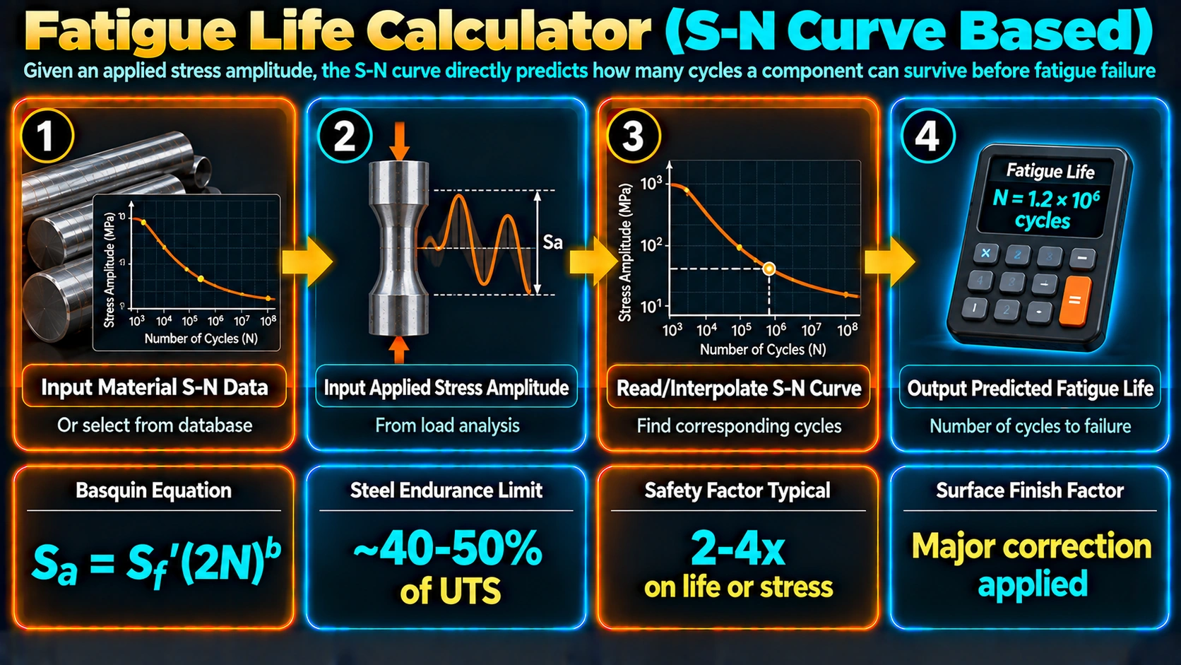
Given two points (S1, N1) and (S2, N2) on a material’s S-N curve, the finite-life region is fitted with a power law of the form S = A × Nb, which becomes a straight line when both axes are plotted logarithmically. Solving for the two constants A and b from the two known points allows the fitted line to be evaluated at any target stress within or reasonably near the range spanned by the input data.
Two-point power law fit:
    S = A x N^b

Taking log of both sides:
    log(S) = log(A) + b x log(N)

Solving for slope b using two points:
    b = [log(S2) - log(S1)] / [log(N2) - log(N1)]

Solving for A:
    log(A) = log(S1) - b x log(N1)

Predicting N at a target stress S_target:
    N = (S_target / A)^(1/b)
3. Basquin’s Equation Method
Basquin’s equation is the standard stress-based fatigue life relationship used throughout high-cycle fatigue analysis, expressing stress amplitude as a function of reversals to failure using two material-specific fatigue properties: the fatigue strength coefficient (σf’, approximately equal to the true fracture stress for many metals) and the fatigue strength exponent (b, typically a small negative number, commonly in the range of about -0.05 to -0.12 for structural metals).
Basquin's equation:
    Sa = sigma_f' x (2Nf)^b

  where Sa      = stress amplitude
        sigma_f' = fatigue strength coefficient
        Nf      = cycles to failure
        2Nf     = reversals to failure (2 reversals per cycle)
        b       = fatigue strength exponent (negative)

Solving for Nf given a target Sa:
    2Nf = (Sa / sigma_f')^(1/b)
    Nf  = 2Nf / 2
4. Interpreting the Fatigue Strength Exponent
The magnitude of b controls how steeply the S-N curve slopes: a larger negative b means life drops off faster for a given increase in stress, while a smaller magnitude b indicates a shallower, more gradual curve. This exponent is closely tied to the material’s cyclic deformation behaviour, which in turn connects back to the same strain-hardening and microstructural concepts discussed in the site’s hardness and mechanical testing coverage — a material with a finer, more homogeneous microstructure often shows more consistent, better-behaved S-N data than one with coarse or heterogeneous microstructure.
5. Why the Fatigue Limit Matters
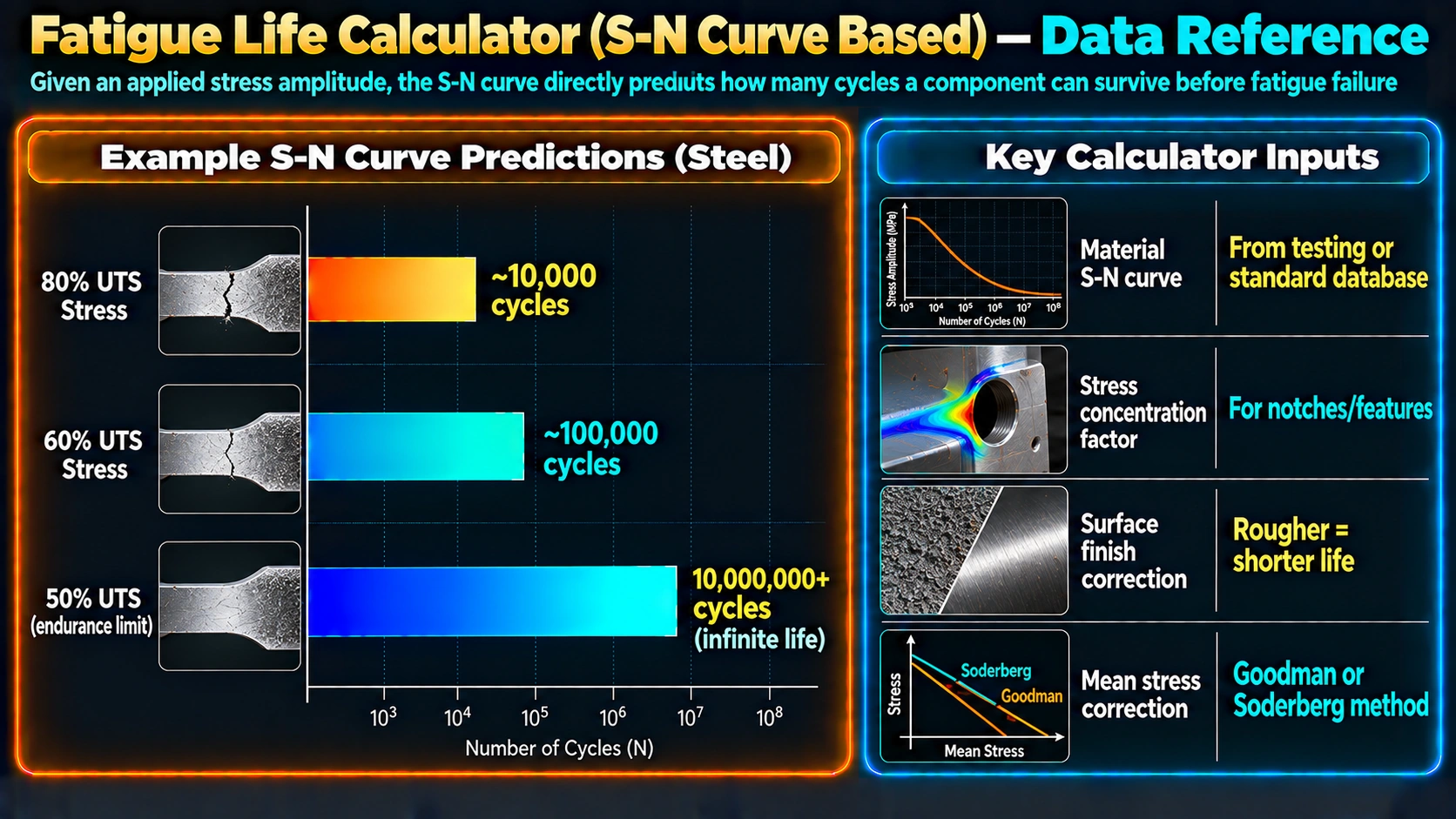
Many carbon and low-alloy steels display a distinct fatigue (endurance) limit — a stress level, typically reached somewhere around 106 to 107 cycles, below which the material can theoretically sustain an effectively unlimited number of cycles without failure. This calculator’s power-law fit follows only the sloped, finite-life portion of the curve and does not automatically detect or apply a fatigue limit plateau, so a predicted life at very low target stress from either mode should be treated as a rough extrapolation rather than a reliable estimate near or below the material’s actual fatigue limit. Many non-ferrous alloys, including most aluminum alloys, do not exhibit a true fatigue limit at all and instead continue a gradually sloping S-N curve indefinitely, which is a separate reason to treat extrapolated results with appropriate caution.
6. Cumulative Damage and Miner’s Rule
Real service loading rarely occurs at a single constant stress amplitude. Where a component experiences several distinct stress levels over its life — for example, different stress amplitudes corresponding to different operating conditions — the individual life predictions from an S-N curve at each stress level are typically combined using Miner’s rule (the linear damage hypothesis), which sums the fraction of life consumed at each stress level and predicts failure when that sum reaches unity.
Miner's rule (linear cumulative damage):

    D = sum( n_i / N_i )   for i = 1 to k stress levels

  where n_i = number of cycles applied at stress level i
        N_i = cycles to failure at stress level i (from
              the S-N curve, e.g. via this calculator)

Failure is predicted when D >= 1.0

Note: Miner's rule is a widely used approximation with
known limitations (it ignores load sequence effects), not
an exact physical law — treat results as a design guide,
not a guarantee.
This calculator computes life at a single stress level; combining multiple levels into a Miner’s rule damage sum is a manual next step using the Nf values this tool produces for each individual load case.
7. Sources of Scatter and Uncertainty
| Factor | Effect on Fatigue Life |
|---|---|
| Surface finish | Rougher surfaces provide more crack initiation sites, reducing life |
| Residual stress | Compressive residual stress (e.g. from shot peening) can substantially extend life; tensile residual stress reduces it |
| Mean stress | Tensile mean stress reduces fatigue life relative to fully reversed loading at the same amplitude |
| Environment | Corrosive or high-temperature environments can significantly reduce life versus lab-air test data |
| Specimen-to-specimen variability | Even nominally identical specimens commonly show an order of magnitude scatter in cycles at a given stress |
Because of this inherent scatter, S-N curve based predictions — including the results from this calculator — are best applied as a comparative or preliminary design tool, with appropriate safety factors applied per the governing design code, rather than treated as a precise forecast of when an individual component will fail.
8. Industrial Applications and Significance
S-N curve based fatigue life estimation underpins design decisions across structural, automotive, aerospace, and offshore engineering — anywhere a component experiences repeated cyclic loading over its service life, from a welded structural connection (see the fatigue design discussion in the site’s offshore structural steel requirements article) to a rotating machine shaft. Understanding both methods this calculator implements, and equally understanding their limitations around the fatigue limit and scatter, is essential for using S-N data responsibly rather than treating a single calculated number as a guarantee.
9. Frequently Asked Questions
What is an S-N curve?
How does the two-point method in this calculator work?
What is Basquin’s equation and when should I use it instead of the two-point method?
Why is fatigue life predicted on a log-log basis rather than a linear scale?
What is a fatigue limit and does this calculator account for it?
Can this calculator be used for variable-amplitude loading?
What units does the calculator use for stress?
How accurate is a fatigue life estimate from an S-N curve?
Recommended Reference Materials
Fatigue of Materials and Structures Handbook
Comprehensive reference on S-N curves, Basquin’s equation, and damage accumulation.
View on AmazonMechanical Behavior of Materials Textbook
Foundational coverage of fatigue theory, cyclic stress-strain response, and Miner’s rule.
View on AmazonASM Handbook — Fatigue and Fracture
In-depth reference data and testing methodology for fatigue property determination.
View on AmazonFatigue Design of Welded Steel Structures
S-N curve application to welded connections and structural fatigue detailing.
View on AmazonDisclosure: MetallurgyZone participates in the Amazon Associates programme. If you purchase through these links, we may earn a small commission at no extra cost to you. This helps support free technical content on this site.
Further Reading
