Fatigue Testing and S-N Curves: Metal Fatigue Explained for Engineers
Metal fatigue is responsible for more in-service structural failures than any other single damage mechanism — responsible for an estimated 50–90% of all mechanical failures across aerospace, automotive, power generation, and offshore industries. This article provides a rigorous, graduate-level treatment of fatigue testing methodology, S-N curve construction, mean stress corrections, notch effects, crack propagation, and the design strategies engineers use to extend fatigue life in critical components.
Key Takeaways
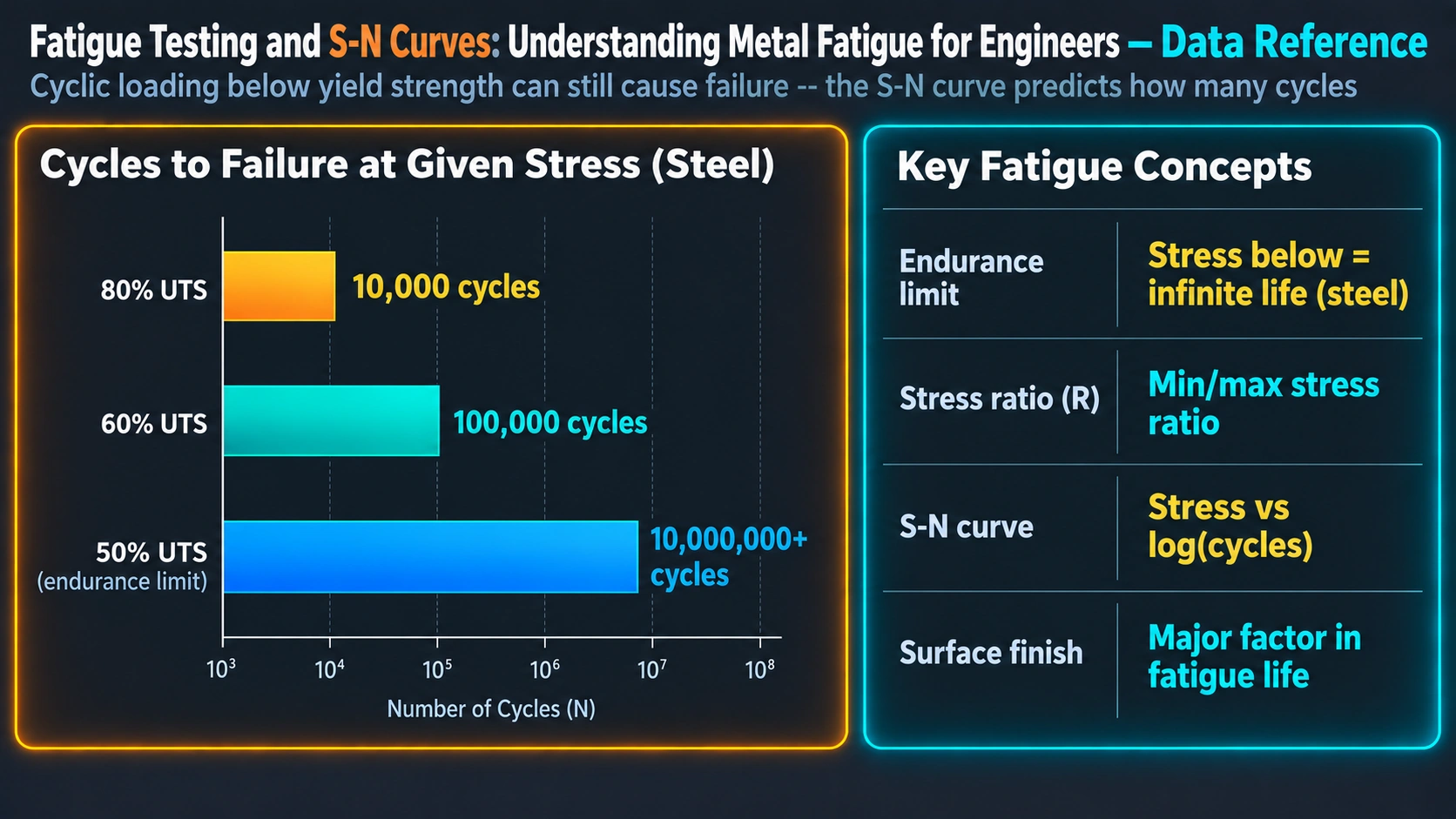
- The S-N (Wöhler) curve defines the relationship between cyclic stress amplitude and cycles to failure; ferritic steels exhibit a distinct endurance limit (~0.4–0.5 × UTS) while aluminium alloys do not.
- The stress ratio R = σmin/σmax characterises the loading cycle; tensile mean stress (R > −1) reduces fatigue life and must be corrected using the Goodman, Gerber, or Soderberg criterion.
- Stress concentrations are quantified by Kt (elastic) and Kf (fatigue notch factor); high-strength steels are more notch-sensitive than low-strength steels, making finish quality critical in high-strength designs.
- Fatigue crack growth in Region II follows the Paris-Erdogan law: da/dN = C(ΔK)m; the exponent m is 2–4 for most structural metals.
- Compressive residual stresses from shot peening, carburising, or nitriding significantly extend fatigue life by retarding crack initiation at the surface.
- Variable amplitude fatigue is assessed using Miner’s linear damage rule; however, load sequence effects mean the rule is only approximate (experimental failure typically occurs at D = 0.7–2.2).
S-N Fatigue Life Estimator
Estimate allowable stress amplitude and cycles to failure using a modified Basquin power-law S-N model with Goodman mean stress correction and surface/notch modifiers.
What is Metal Fatigue?
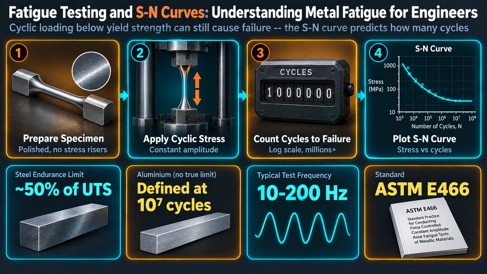
Fatigue is the progressive, localised, and permanent structural damage that occurs when a material is subjected to cyclic or fluctuating stresses below its static yield strength. The underlying mechanism proceeds in three distinct stages: (I) crack initiation at a surface discontinuity, stress concentration, or persistent slip band; (II) stable crack propagation under cyclic loading; and (III) sudden fracture when the remaining cross-section can no longer sustain the applied load.
The defining characteristic of fatigue failure is that it occurs at stresses far below the material’s monotonic yield or ultimate tensile strength — a fact that makes it uniquely dangerous in engineering structures subjected to vibration, rotating loading, thermal cycling, or pressure fluctuations. Fatigue fracture surfaces exhibit characteristic macroscopic features: a smooth, “clamshell” beach mark region representing stable crack growth, and a rough, fibrous or granular region representing final fast fracture.
Cyclic Stress Terminology and the Stress Ratio
Before interpreting an S-N curve, understanding the standard stress cycle descriptors is essential. For a sinusoidal cycle with maximum stress σmax and minimum stress σmin:
Stress amplitude:   σ_a = (σ_max − σ_min) / 2
Mean stress:        σ_m = (σ_max + σ_min) / 2
Stress range:       Δσ  = σ_max − σ_min = 2σ_a
Stress ratio:       R   = σ_min / σ_max
Amplitude ratio:    A   = σ_a / σ_m
The stress ratio R defines the loading character:
| R value | Loading type | Mean stress | Typical application |
|---|---|---|---|
| R = −1 | Fully reversed | σm = 0 | Rotating beam test; bending fatigue |
| R = 0 | Pulsating tension | σm = σa | Pressurised vessels; axial pulsation |
| 0 < R < 1 | Tensile mean, partial unload | Tensile | Press fits; bolt fatigue under preload |
| R = +1 | Static load (no cycle) | Equal max/min | No fatigue damage |
| −∞ < R < −1 | Fully reversed with compressive mean | Compressive | Compression springs; rail head |
Standard S-N data is almost always generated at R = −1. Correcting to other R ratios requires mean stress correction models discussed in the section on the Goodman diagram.
The S-N Curve: Construction and Interpretation
Wöhler (Rotating Beam) Testing
The classical rotating beam fatigue machine (Moore-type, ASTM E466/E468) subjects a polished, hourglass-section specimen to a four-point or cantilever bending moment while rotating at constant speed. Because the specimen rotates in a constant bending field, every surface fibre experiences one complete sinusoidal stress cycle per revolution — a fully reversed (R = −1) loading at the target frequency (typically 3000–10,000 rpm).
A minimum of one specimen per stress level is tested. Modern practice per ASTM E739 and ISO 12107 requires:
- At least 6 specimens for a preliminary or research-grade curve.
- 12–24 specimens for a definitive design S-N curve at each stress level.
- Statistical treatment to produce P-S-N (probability-stress-life) curves, most commonly at 50% and 90% survival probability.
Axial and Servo-Hydraulic Testing
For axial push-pull testing (ASTM E466), servo-hydraulic or linear resonance machines apply controlled force or displacement amplitudes. Axial test data is approximately 15% lower than rotating beam data for the same nominal stress amplitude, because the volume of highly stressed material is larger in axial loading. The endurance limit in axial loading is typically corrected by a loading factor ka = 0.85 relative to rotating bending.
Endurance Limit and Fatigue Strength
Ferritic (body-centred cubic, BCC) steels and some titanium alloys display a genuine endurance limit — a stress amplitude below which fatigue crack initiation does not occur for an effectively infinite number of cycles (>107). The endurance limit Se‘ of a polished steel specimen under rotating bending can be approximated from the ultimate tensile strength:
For UTS ≤ 1400 MPa:    S_e' ≈ 0.504 × UTS     (Shigley empirical approximation)
For UTS > 1400 MPa:    S_e' ≈ 700 MPa          (plateau — ceases to increase)
This approximation is useful only for smooth, polished specimens. The design endurance limit Se must be obtained by applying correction factors:
S_e = k_a × k_b × k_c × k_d × k_e × S_e'

Where:
  k_a = surface condition factor     (polished → as-forged: 0.9 → 0.45)
  k_b = size factor                  (d < 8 mm: 1.0; d > 50 mm: ~0.75)
  k_c = load type factor             (bending: 1.0; axial: 0.85; torsion: 0.59)
  k_d = temperature factor           (≤450°C: 1.0; higher: reduces)
  k_e = reliability factor           (50%: 1.0; 99%: 0.814)
Aluminium alloys, copper alloys, and most non-ferrous metals have no endurance limit. Their S-N curves continue declining through 108 and beyond. The “fatigue strength at N cycles” (commonly 108 for aluminium) is specified instead, and design must explicitly define the intended service life.
Basquin’s Power Law
The finite life region of an S-N curve (typically 103–107 cycles) is well described by Basquin’s equation:
σ_a = σ_f' × (2N)^b

Where:
  σ_a   = stress amplitude (MPa)
  σ_f'  = fatigue strength coefficient ≈ UTS to 1.5×UTS (material constant)
  b     = Basquin exponent (fatigue strength exponent) — typically −0.05 to −0.12
  N     = cycles to failure
  2N    = reversals to failure (one reversal = half-cycle)
Rearranging to solve for life at a given stress amplitude:
log N = (log(σ_f') − log(σ_a)) / b   or equivalently

N = (σ_a / σ_f')^(1/b) / 2
Low Cycle vs High Cycle Fatigue
The boundary between low cycle fatigue (LCF) and high cycle fatigue (HCF) is conventionally set at approximately 104–105 cycles:
| Regime | Cycle range | Dominant variable | Governing equation | Typical examples |
|---|---|---|---|---|
| LCF | 102–104 | Plastic strain amplitude | Coffin-Manson: Δεp/2 = εf‘(2N)c | Turbine disc, pressure vessel pressure cycles |
| HCF | 105–108 | Stress amplitude | Basquin: σa = σf‘(2N)b | Rotating shafts, springs, gears |
| VHCF | >108 | Internal inclusions; sub-surface | Fish-eye crack initiation model | Ultrasonic fatigue; bearing races |
In LCF, significant plastic deformation occurs each cycle; the Coffin-Manson relationship governs because the strain amplitude is the controlling variable. The combined Basquin-Coffin-Manson (total strain-life) equation covers both regimes:
Δε_total / 2 = (σ_f' / E)(2N)^b  +  ε_f'(2N)^c

Where:
  σ_f'/E  = elastic strain amplitude term
  ε_f'    = fatigue ductility coefficient
  c       = fatigue ductility exponent (typically −0.5 to −0.7)
  E       = Young's modulus (MPa)
The crossover point (where elastic and plastic strain amplitudes are equal) defines the transition life NT. Materials to the right of NT favour high-strength (HCF regime); to the left, high ductility (LCF regime).
Mean Stress Effects and the Goodman Diagram
S-N data generated at R = −1 applies only to components where the mean stress is zero. Most real components operate with a significant tensile mean stress (e.g., rotating shaft under gravitational load, bolt under preload, pressurised pipe). Tensile mean stress is detrimental because it promotes crack opening and accelerates propagation.
Modified Goodman Criterion
The most widely used mean stress correction in engineering design is the modified Goodman criterion:
σ_a / S_e  +  σ_m / UTS  =  1

Rearranged for allowable amplitude:
σ_a,allow = S_e × (1 − σ_m / UTS)

Safety factor against fatigue:
SF = 1 / (σ_a/S_e + σ_m/UTS)
The Goodman line connects Se on the stress amplitude axis to UTS on the mean stress axis. Operating points below the line are safe in fatigue; above the line, fatigue failure is predicted within the design life. Note that yield must also be checked: the Langer static yield line (Sy = σa + σm) defines the boundary beyond which first-cycle yielding occurs.
Gerber and Soderberg Criteria
The Gerber criterion uses a parabolic correction:
σ_a / S_e + (σ_m / UTS)² = 1
Gerber is less conservative than Goodman and better fits many experimental datasets for ductile metals under tensile mean stress. The Soderberg criterion replaces UTS with yield strength Sy, making it the most conservative:
σ_a / S_e + σ_m / S_y = 1
In practice, the modified Goodman criterion is preferred for most engineering design because it balances conservatism and accuracy. For welded joints, the FAT class system (IIW recommendations) implicitly includes mean stress effects through weld-specific S-N curves that account for the high tensile residual stresses inherent to welds.
Stress Concentration and Notch Effects
Virtually all practical engineering components contain geometric discontinuities — notches, holes, fillets, keyways, threads, press-fit interfaces, and weld toes. These create local stress amplification that dramatically reduces fatigue life relative to smooth specimens. Understanding the relationship between the elastic stress concentration factor Kt and the fatigue notch factor Kf is essential for hardness-sensitive materials design.
Elastic Stress Concentration Factor Kt
Kt is defined as the ratio of the peak local stress to the nominal applied stress:
K_t = σ_max,local / σ_nominal
Kt is a purely geometric parameter, independent of material, determined by the notch geometry (notch root radius r, notch depth d, specimen width W). Charts in Peterson’s Stress Concentration Factors or closed-form solutions provide Kt for standard geometries. Finite element analysis is used for complex geometries.
Fatigue Notch Factor Kf and Notch Sensitivity
The fatigue notch factor Kf is defined as:
K_f = (endurance limit of smooth specimen) / (endurance limit of notched specimen)
K_f = 1 + q(K_t − 1)

Where q = notch sensitivity index:
  q → 0: material is notch-insensitive (local plasticity blunts stress concentration)
  q → 1: material is fully notch-sensitive (endurance limit reduced by full K_t factor)

Neuber approximation for q:
  q = 1 / (1 + √(a_N/r))

Where a_N = Neuber's material constant (function of UTS):
  Steel at 700 MPa UTS:   a_N ≈ 0.25 mm
  Steel at 1000 MPa UTS:  a_N ≈ 0.08 mm
  Steel at 1400 MPa UTS:  a_N ≈ 0.02 mm
  Al alloys:              a_N ≈ 0.6–1.5 mm
Fatigue Crack Initiation Mechanisms
Understanding where and why fatigue cracks initiate is fundamental to prevention. In smooth, clean metallic specimens, initiation occurs through persistent slip band (PSB) formation: localised cyclic plastic deformation concentrates slip on specific crystallographic planes, forming extrusions and intrusions at the free surface that act as micro-notches after extended cycling. Once a micro-crack of critical depth forms (typically 10–100 μm), it transitions to Stage II growth controlled by the stress intensity factor range ΔK.
In engineering components, initiation is almost always dominated by one of the following:
- Surface roughness and machining marks: Each machining groove acts as a shallow notch. As-forged or shot-blasted surfaces have fatigue strength 40–55% lower than polished surfaces at high UTS levels.
- Metallurgical inclusions: Non-metallic inclusions (MnS stringers, oxide clusters, TiN cuboids in bearing steels) act as stress concentrators and debond from the matrix under cyclic loading. In very high cycle fatigue (>108), subsurface inclusion-initiated “fish-eye” cracks dominate failure even when the surface is pristine.
- Corrosion pits: Even shallow corrosion pits (depth 10–100 μm) effectively eliminate the endurance limit of steel in corrosive environments by providing pre-existing sharp notches.
- Welding defects and weld toe geometry: Weld toes combine a geometric notch (Kt = 2–4 depending on weld profile) with residual tensile stresses, making welded joints the most fatigue-sensitive element in many fabricated structures. See the MetallurgyZone guide to HAZ microstructure and its mechanical consequences.
- Press fits and fretting: Interference-fit interfaces develop fretting damage — micro-slip and oxide debris formation — that dramatically nucleates fatigue cracks at the contact boundary (locomotive axle fits, turbine blade roots).
Fatigue Crack Propagation: Paris Law and Fracture Mechanics
Once a crack has initiated and exceeded the threshold stress intensity factor range ΔKth, it enters the stable propagation regime governed by linear elastic fracture mechanics (LEFM). The stress intensity factor range is:
ΔK = K_max − K_min = Y × Δσ × √(πa)

Where:
  Y     = geometry correction factor (dimensionless; tabulated for crack/specimen geometries)
  Δσ    = applied stress range (MPa)
  a     = current crack half-length (m)
  ΔK in MPa√m
The Paris-Erdogan law (1963) describes crack growth per cycle in Region II:
da/dN = C × (ΔK)^m

Where:
  da/dN = crack extension per cycle (m/cycle)
  C, m  = material constants (determined from crack growth testing per ASTM E647)

Typical values:
  Structural steels:   C ≈ 6×10⁻¹² m/cycle, m ≈ 3.0
  Austenitic stainless: C ≈ 5×10⁻¹², m ≈ 3.3
  Al 2024-T3:          C ≈ 5×10⁻¹¹, m ≈ 3.5
  Ti-6Al-4V:           C ≈ 1×10⁻¹¹, m ≈ 3.4
Integrating the Paris equation from initial crack size ai to critical crack size af (where Kmax = KIC) gives the number of cycles to fracture:
For m ≠ 2:
N_f = [a_f^(1−m/2) − a_i^(1−m/2)] / [C × (Y×Δσ×√π)^m × (1−m/2)]

Critical crack size a_f:
a_f = (1/π) × (K_IC / (Y × σ_max))²
This damage-tolerant approach — which underpins aircraft structural inspection intervals, pressure vessel fitness-for-service assessment (API 579/ASME FFS-1), and offshore platform inspection scheduling — requires knowledge of the initial defect size from non-destructive examination, the crack growth constants C and m, and the material fracture toughness KIC. See the Charpy impact test and fracture toughness article for toughness characterisation.
Crack Closure and Effective ΔK
Elber (1970) demonstrated that fatigue cracks close at positive stress intensities during unloading, reducing the effective driving force for crack growth. The effective stress intensity factor range ΔKeff = Kmax − Kop (where Kop is the crack opening stress intensity) governs the actual crack advance per cycle. Compressive residual stresses enhance crack closure (beneficial); tensile residual stresses reduce it (detrimental). The plasticity-induced crack closure concept explains why shot peening or laser peening extends fatigue life substantially beyond what a simple surface finish improvement would provide.
Variable Amplitude Fatigue and Damage Accumulation
Real service loading is rarely constant amplitude. Aircraft wings, crane hooks, automotive suspension components, and offshore risers all experience irregular, spectrum load histories. Handling variable amplitude fatigue requires a damage accumulation rule.
Miner’s Rule
D = Σ (n_i / N_fi)   →   Failure when D = 1.0

Where:
  n_i   = number of cycles applied at stress level i
  N_fi  = cycles to failure at stress level i (from S-N curve)
  D     = cumulative Miner damage sum
Miner’s rule assumes linear damage accumulation and independence of loading sequence. Experimental failure occurs over D ≈ 0.7–2.2, with the majority of datasets clustering near D = 1 ± 0.5. High-to-low sequence loading (starting with the highest amplitude) tends to give D < 1 at failure (crack initiation and early propagation occur early, consuming more life); low-to-high sequence loading tends to give D > 1 (compressive residual stresses introduced by early low-amplitude cycles crack tip blunting). For design, a Miner sum limit of D = 0.5–0.7 is used in critical applications to account for this scatter.
Rainflow Cycle Counting
For complex irregular load histories, the rainflow counting method (ASTM E1049) extracts individual stress cycles from the time history. The method identifies closed hysteresis loops in the stress-strain plane, correctly handling the influence of large infrequent cycles on smaller background cycles. The output is a cycle count matrix (amplitude versus mean) that feeds directly into Miner’s rule and Goodman corrections.
Fatigue in Welds: Special Considerations
Welded joints introduce three simultaneous penalties that make them the most fatigue-critical detail in most fabricated structures:
- Geometric stress concentration: The weld toe acts as a sharp notch (Kt = 1.5–3.5 depending on weld profile angle and toe radius).
- Tensile residual stresses: Weld shrinkage leaves tensile residual stresses at the toe approaching yield strength, equivalent to operating at high positive mean stress regardless of the applied loading R ratio.
- Metallurgical damage: The heat-affected zone may contain coarse-grained regions of reduced toughness, and hydrogen absorbed during welding can accelerate crack propagation if not removed by post-weld heat treatment. See the MetallurgyZone article on hydrogen-induced cracking for this interaction.
Weld fatigue design is typically based on structural hot-spot stress or effective notch stress approaches, with FAT classes (IIW/ISO 5817) specifying S-N curves at specific survival probabilities for each joint detail category. Post-weld improvement techniques — TIG dressing, burr grinding, hammer peening, and high-frequency mechanical impact (HFMI) — can raise a weld detail by one to two FAT classes by improving toe geometry and introducing compressive residual stresses.
Improving Fatigue Life: Engineering Strategies
Surface Treatments
Because fatigue cracks almost always initiate at the free surface, surface engineering is the most effective lever for improving fatigue performance:
| Treatment | Mechanism | Typical life improvement | Applications |
|---|---|---|---|
| Shot peening | Compressive residual stress, strain hardening | 20–200% increase | Springs, gears, aircraft structure |
| Laser peening | Deep compressive residual stress (2–5 mm vs. 0.2–0.5 mm for shot) | 2–5× increase | Turbine blades, aerostructures |
| Carburising / nitriding | Hard case + compressive residual stress from transformation expansion | 50–200% | Gears, crankshafts, camshafts |
| Case hardening (induction) | Surface martensite with compressive residual stresses | 30–100% | Shafts, races, axles |
| Cold rolling (fillet rolling) | Compressive residual stress at fillet radii | 50–200% | Crankshaft fillets, rail |
| Electropolishing / mirror finish | Eliminates stress-concentrating surface roughness | 10–40% | Medical implants, aerospace fasteners |
The heat treatment interplay with fatigue is reviewed in the quenching and tempering and annealing and normalising guides on MetallurgyZone. The martensite formation article explains why the volumetric expansion associated with martensite transformation is the source of beneficial compressive surface stresses in case-hardened components.
Design Geometry Optimisation
- Maximise fillet radii at stress raisers: doubling a fillet radius from 1 mm to 2 mm can reduce Kt from 2.5 to 1.8 at the same stress gradient.
- Avoid abrupt cross-section changes; taper transitions reduce Kt.
- For threaded fasteners, rolled threads (compressive residual stress) outperform cut threads by 20–40% in fatigue life.
- Avoid eccentricity in load paths that introduces unintended bending into nominally axial components.
Material Selection
For HCF-dominated applications, maximising UTS (and thus Se) is often the starting point, but notch sensitivity must be factored in. Bainitic steels offer attractive combinations of strength, toughness, and lower notch sensitivity compared to fully martensitic steels at equivalent hardness. For corrosion fatigue environments, material selection for corrosion resistance (duplex stainless, titanium) or protective coatings (thermal spray, cadmium for aerospace) is prioritised over UTS maximisation.
Corrosion Fatigue and Environmental Effects
When cyclic loading occurs in a corrosive environment (sea water, dilute acids, moist air), corrosion fatigue dramatically reduces fatigue life. The endurance limit of steel effectively disappears in salt water, and the fatigue strength at 108 cycles is typically 25–50% of the air value. The mechanisms include:
- Pitting provides pre-initiated cracks, bypassing the initiation stage.
- Dissolution of protective oxide films at the crack tip prevents oxide-induced crack closure, increasing ΔKeff.
- Hydrogen embrittlement at crack tips (anodic dissolution produces hydrogen) accelerates crack growth in high-strength steels. This is discussed in the corrosion mechanisms article.
- Frequency effect: lower cycling frequencies expose the crack tip to the environment for longer per cycle, increasing corrosion fatigue crack growth rates at low frequencies.
Design for corrosion fatigue requires a combination of material selection (corrosion-resistant alloys), protective coatings (cadmium, zinc, epoxy), cathodic protection (for marine structures), shot peening (compressive stresses that slow pit-to-crack transition), and corrosion-allowance margins in S-N data selection. Refer to the MetallurgyZone article on pitting corrosion for the electrochemical context.
Industrial Applications and Standards
Aerospace
Fatigue is the primary certification driver for metallic airframes. The damage-tolerant design philosophy (MIL-STD-1530, FAR 25.571) requires demonstration that a structure can sustain a defined crack size without failing for two inspection intervals. NASGRO, AFGROW, and DARWIN software implement Paris-law crack growth with closure correction across complex spectrum load histories. Shot peening, laser peening, and cold worked fastener holes are mandatory treatments on primary structure.
Power Generation
Steam turbine discs and blades, gas turbine compressor blades, and nuclear reactor pressure vessels all require rigorous fatigue assessment. ASME Section VIII Div. 2 (pressure vessels) and ASME Section III (nuclear) provide design fatigue curves, with explicit penalties for surface finish, mean stress, and environment. The creep-fatigue interaction (important above 550–600°C in power generation components) is discussed in the creep testing and stress rupture article.
Automotive
Automotive fatigue assessment typically uses the local strain approach (strain-life method) rather than the nominal stress S-N approach, because the high-cycle regime is less relevant than the LCF regime in suspension and powertrain components. IATF 16949 statistical process control governs heat treatment and surface treatment processes that determine fatigue performance.
Offshore Structures and Pipelines
Wave-loading on fixed offshore platforms and fatigue of risers and mooring chains is assessed per DNV-RP-C203 and API RP 2A. The guidance uses structural hot-spot stress S-N curves with explicit seawater knockdown factors. Inspection intervals are set using fracture mechanics crack growth calculations from the assumed initial weld defect size.
Frequently Asked Questions
What is the endurance limit and which metals exhibit it?
How is an S-N curve generated experimentally?
What is the stress ratio R and how does it affect fatigue life?
How do stress concentrations affect fatigue strength?
What is the Paris law and what does the exponent m indicate?
What surface treatments most effectively improve fatigue life?
How does corrosion fatigue differ from air fatigue?
What is the Goodman diagram and how is it applied in design?
What is Miner’s rule and what are its known limitations?
How many specimens are needed for a statistically valid S-N curve?
Recommended References
Disclosure: MetallurgyZone participates in the Amazon Associates programme. If you purchase through these links, we may earn a small commission at no extra cost to you. This helps support free technical content on this site.
Further Reading
